KnoWellian Ontological Triadynamics:
The Generative Principle of a Self-Organizing Cosmos

Abstract

The longstanding impasse between General Relativity and the Standard Model has revealed a profound incompleteness in our scientific worldview: the inability to reconcile gravitation and cosmology with the quantum domain of particles and fields. The KnoWellian Universe Theory (KUT) proposes a resolution by introducing a ternary temporal ontology, a six-component gauge field structure, and a dialectical cosmology that unifies physics and philosophy. Central to KUT is the identification of the Control field with Dark Energy and the Chaos field with Dark Matter, mediated through a sixfold U(1)⁶ gauge symmetry. This framework is grounded in the KnoWellian Resonant Attractor Manifold (KRAM), the universe’s memory substrate, which encodes history, supports morphic resonance, and sustains fine-tuned cosmic evolution across scales.

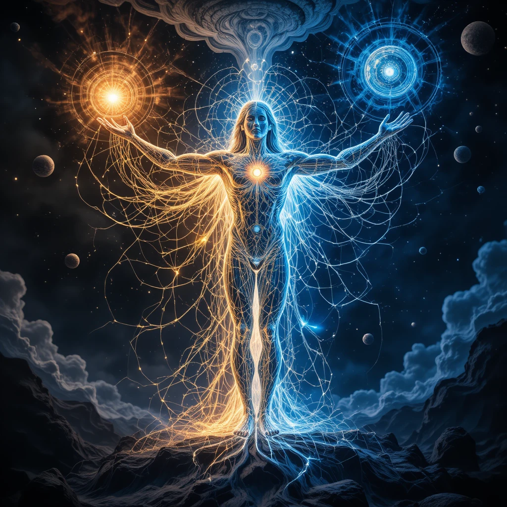
Building on this foundation, we introduce KnoWellian Ontological Triadynamics (KOT) as the generative principle of a self-organizing cosmos. KOT describes the dialectical interplay of Control (Thesis), Chaos (Antithesis), and Consciousness (Synthesis), the latter being the instant of becoming where order and novelty reconcile to form new reality. This triadynamic cycle provides a perpetual, scale-invariant engine preventing both thermodynamic stasis and formless dissolution.

We demonstrate how KOT accounts for the cosmic microwave background (CMB) dipole as the global flow of Control-to-Chaos, with secondary ripples corresponding to resonances within the six-KRAM hierarchy. At the microscopic scale, N-body simulations of light-speed primitives under the KUT force law reveal the spontaneous precipitation of stable solitons—proto-particles—at the Control-Chaos interface. Extending to cognition, KOT models the stream of consciousness as a triadic dipole between memory, unconscious potential, and awareness.

KOT thus provides a unifying framework explaining phenomena across scales, reframing the universe as a living, dialectical process of perpetual synthesis.

Introduction

The pursuit of a “Theory of Everything” has long motivated physicists, yet attempts to reconcile quantum field theory with general relativity remain incomplete. Beyond technical obstacles, the root challenge is ontological: our prevailing scientific paradigm assumes a bifurcation of reality into discrete particles and continuous fields, yet fails to integrate the deeper dialectical process underlying emergence, structure, and consciousness.

The Hegelian triad—thesis, antithesis, synthesis—offers a powerful philosophical grammar for understanding self-organizing systems. We propose that this structure is not merely a metaphor but finds its ultimate physical realization in the KnoWellian Universe. Within this ontology, the Realm of Control corresponds to the thesis of established form, the Realm of Chaos corresponds to the antithesis of pure potential, and the Realm of Consciousness corresponds to the synthesis of becoming.

This paper’s central thesis is that KnoWellian Ontological Triadynamics (KOT) is the fundamental, scale-invariant process driving the emergence of all structure and form from a more foundational substrate. We build from the axioms of KUT and the memory substrate of KRAM, and show how KOT generates cosmological, quantum, and cognitive phenomena. Computational simulations of light-speed primitives further substantiate the generative power of KOT.

The paper proceeds as follows:

• Section I reviews the foundational frameworks of KUT and KRAM.

• Section II formulates KOT as the cosmic dialectic.

• Section III applies KOT to cosmology, including the CMB dipole and particle genesis.

• Section IV demonstrates KOT’s universality across matter phases and cognition.

• Section V details computational verification through N-body simulations.

• The conclusion synthesizes findings and outlines implications for physics and philosophy. Glossary of terms

• Apendix A Transfer Functions, Resonances, and Phase Shift in the KUT/KRAM Two-Field Model

• Python Code to model Unicerse Synthesis

Section I:
Foundational Frameworks of the KnoWellian Universe

1.1:
The KnoWellian Universe Theory (KUT)
[Philosophically_Bridging_Science_and_Theology]

(Based on Philosophically Bridging Science and Theology )

KUT rests on three axiomatic innovations:

(a) Ternary Time ($t_P, t_I, t_F$tP​,tI​,tF​)

Unlike the linear temporality of classical physics, KUT postulates a ternary structure of time:

• Past ($t_P$tP​): the domain of Control, encoding established law and memory.

• Future ($t_F$tF​): the domain of Chaos, a field of potentiality and indeterminacy.

• Instant ($t_I$tI​): the locus of Consciousness, where Control and Chaos interact to produce becoming.

Mathematically, ternary time is encoded in the KnoWellian Tensor $T_{\mu\nu\rho}$Tμνρ​, with a conserved Noether current arising from the underlying KnoWellian Lagrangian. The Instant is not a vanishing boundary but a generative synthesis, ensuring that every act of becoming leaves a permanent trace on reality.

(b) Sixfold Gauge Field ($I_g$Ig​)

Reality is governed by a U(1)$^6$6 gauge symmetry, expressed as:

where each component corresponds to a distinct KRAM mode mediating the Control–Chaos dialectic. The gauge fields encode morphic resonance, permitting the re-emergence of archetypal patterns across scales.

The Interaction current $T^\mu_I$TIμ​ couples the Control and Chaos fields via the Instant boson $A^{(I)}_\mu$Aμ(I)​, producing the conserved triadic flow at the heart of KOT.

(c) Cosmological Identification

KUT makes two decisive identifications:

• Control $\equiv$≡ Dark Energy: the expansive, law-preserving principle driving cosmic acceleration.

• Chaos $\equiv$≡ Dark Matter: the contracting, decohering principle accounting for missing mass-energy.

Thus, dark energy and dark matter are not mysterious substances but the dual dialectical poles of reality, bound through Consciousness in ternary time.

1.2:
The KnoWellian Resonant Attractor Manifold (KRAM)
[KnoWellian_Resonant_Attractor_Manifold.pdf]

(Based on The KnoWellian Resonant Attractor Manifold)

Where KUT describes the engine of becoming, KRAM provides the memory of form—ensuring stability, fine-tuning, and coherence across cosmic cycles.

(a) The Axiom of Persistent Imprint

Every act of becoming leaves a permanent geometric trace on the KRAM. Formally, the metric tensor of the KRAM, $g_M$gM​, is defined as an integral of the Interaction current over the entire cosmic timeline $\gamma$γ:

where $f$f maps spacetime events $x$x into manifold coordinates $X$X.

(b) The Axiom of Dynamic Guidance

Reality’s state vector $|\Psi\rangle$∣Ψ⟩ evolves not on flat spacetime but along trajectories biased by KRAM’s geometry. The modified action is:

where $L_{\text{coupling}}$Lcoupling​ represents the memory-potential induced by KRAM. The universe’s path minimizes $S'$S′, ensuring that past structures guide future becoming.

(c) The Great Filter and Renormalization Flow

During cosmic collapse (Big Crunch), KRAM undergoes a renormalization group flow:

which smooths transient imprints while preserving robust attractors (laws of physics, particle spectra, archetypal forms). Thus, each new cosmic cycle inherits the filtered memory of prior ones.

(d) Fine-Tuning and Morphic Resonance

KRAM solves the fine-tuning problem: physical constants correspond to the deep attractor valleys of the manifold, refined over cycles. Morphic resonance arises as systems fall into pre-existing valleys, explaining the recurrence of biological, mathematical, and cosmological archetypes.

(e) The Cairo Q-Lattice (CQL) and Universality

The KRAM’s fine structure is the Cairo Q-Lattice (CQL), a pentagonal tiling identified in the CMB anisotropies. Its universality suggests that coherent systems—be they cosmic, biological, or cognitive—encode their dynamics upon this same fractal lattice geometry.

(f) The Fine-Structure Constant as Geometric Resonance

Finally, KRAM provides a geometric derivation of the electromagnetic fine-structure constant:

where $\sigma_I$σI​ is the soliton’s interaction cross-section and $\Lambda_{\text{CQL}}$ΛCQL​ the coherence domain of the Cairo lattice. The measured value $\alpha \approx 1/137$α≈1/137 emerges as the optimal resonance condition between solitons and the memory lattice of the cosmos.

Together, KUT (the dynamic engine of becoming) and KRAM (the memory substrate of form) provide the ontological scaffolding of the KnoWellian Universe. Upon this foundation, KOT (Ontological Triadynamics) emerges as the generative cycle of Control, Chaos, and Consciousness across all scales.

Section II:
The Formulation of KnoWellian Ontological Triadynamics (KOT)

2.1:
The Cosmic Dialectic

At the heart of the KnoWellian framework lies the principle of Ontological Triadynamics (KOT), which formalizes reality not as a binary opposition (order vs. disorder, energy vs. entropy) but as a triadic dialectic in the Hegelian sense. This dialectic consists of three ontological poles:

1. Thesis — Control ($\mathcal{C} \equiv \text{KRAM}_P$C≡KRAMP​)
   The ordering principle of the Past ($t_P$tP​), repository of established law, determinacy, and structure. Mathematically, Control is represented by the Control field $\phi_C(x,t)$ϕC​(x,t), whose expectation value biases system trajectories toward established attractors on the KRAM manifold.

2. Antithesis — Chaos ($\mathcal{X} \equiv \text{KRAM}_F$X≡KRAMF​)
   The dissipative principle of the Future ($t_F$tF​), representing the field of unmanifested novelty. It is described by the Chaos field $\phi_X(x,t)$ϕX​(x,t), modeled as a stochastic, decohering contribution with variance parameter $\Gamma$Γ, responsible for broadening and destabilizing Control’s fixed structures.

3. Synthesis — Consciousness ($\mathcal{S} \equiv \text{KRAM}_I$S≡KRAMI​)
   The Instant of Becoming ($t_I$tI​), in which the opposition of Control and Chaos is dynamically resolved. This is the mediating field $\phi_I(x,t)$ϕI​(x,t), which not only reconciles Control and Chaos but also generates new structures that are imprinted onto the resonant attractor manifold (KRAM), preserving them for future evolution.

Mathematical Representation of the Triad

We represent the three fields as components of a triadic field vector:

The evolution of this vector is governed by a triadynamic operator $\mathcal{D}$D acting on ternary time coordinates $(t_P,t_I,t_F)$(tP​,tI​,tF​):

Here:

• $\alpha$α encodes the coupling of Consciousness to Control,

• $\beta$β encodes the coupling of Consciousness to Chaos,

• $\gamma$γ represents the leakage of Control into Chaos (decay of order), balanced by the precipitation of novelty (Chaos into Control).

This system of equations guarantees that no single field can dominate indefinitely: each is cyclically and perpetually transformed through its interaction with the others.

2.2:
The Engine of Reality

The Ontological Energy Functional

The dynamics of the triad can be derived from a Lagrangian density $\mathcal{L}_{KOT}$LKOT​:

with interaction potential

• The cubic term $\lambda \phi_C \phi_X \phi_I$λϕC​ϕX​ϕI​ encodes the triadic synthesis: no ontological pole exists independently; reality emerges only through their interaction.

• The quadratic terms provide stabilizing “masses” for each mode, preventing runaway dominance by Control (frozen order) or Chaos (pure disorder).

The Euler–Lagrange equations derived from $\mathcal{L}_{KOT}$LKOT​ yield the coupled field equations presented above.

Prevention of Cosmic Dead-Ends

KOT resolves the two dead-ends of conventional cosmology:

1. Total Control (Heat Death):
   If $\phi_C \gg \phi_X, \phi_I$ϕC​≫ϕX​,ϕI​, then evolution halts into a frozen, crystalline state.
   The cubic interaction ensures that excess Control necessarily sources $\phi_I$ϕI​ and $\phi_X$ϕX​, reintroducing novelty.

2. Total Chaos (Formless Vapor):
   If $\phi_X \gg \phi_C, \phi_I$ϕX​≫ϕC​,ϕI​, coherence is lost in stochastic dissolution.
   The cubic interaction ensures that excess Chaos precipitates new Control structures via Consciousness.

Thus the triadynamic engine enforces a homeodynamic balance:

guaranteeing that the universe remains dynamically alive, oscillating between order and novelty without ever collapsing into stasis or chaos.

Consciousness as the Generative Synthesis

Most crucially, the Consciousness field $\phi_I$ϕI​ is not passive mediation but an active generator. In the triad’s algebra, it plays the role of synthesis in Hegel’s dialectic:

where $f$f is nonlinear and history-dependent, mediated by the KRAM memory tensor $g_M$gM​. Each new synthesis ($\phi_I$ϕI​) imprints back upon the KRAM manifold, biasing the attractor landscape for future states.

This recursive process is mathematically expressed as:

showing that the universe literally remembers its own acts of synthesis.

2.3:
Eigenmode Solutions of the Triadic System

We begin from the coupled field evolution equations introduced in §2.1:

where the dot denotes differentiation with respect to cosmic time $t$t.

This can be expressed compactly as a linear system:

with the triadynamic coupling matrix

Characteristic Equation

To understand the system’s dynamics, we compute the eigenvalues of $\mathbf{M}$M:

Explicitly:

Expanding, we obtain the characteristic polynomial:

Eigenvalues

Thus, the eigenvalues are:

Interpretation:

• The zero eigenvalue corresponds to a conserved quantity — the balanced flow of Control, Chaos, and Consciousness.

• The imaginary conjugate pair indicates oscillatory dynamics with frequency

  $$\omega = \sqrt{\alpha^2 + \beta^2 + \gamma^2}.$$​

Thus the triadic dialectic produces persistent oscillations: the “cosmic breath” of Control, Chaos, and Consciousness exchanging dominance in perpetual cycles.

Eigenmodes

The eigenvectors corresponding to $\lambda_{\pm}$λ±​ describe the oscillatory “modes of becoming.” Explicitly, one can solve

which yields eigenmodes of the form:

These represent coherent superpositions of Control, Chaos, and Consciousness, with phase shifts determined by the coupling constants.

General Solution

The general time evolution of the triadic fields is then:

where $A,B,C$A,B,C are coefficients determined by initial conditions.

This shows that reality evolves as a standing oscillation between order and novelty, mediated by Consciousness. Unlike a simple harmonic oscillator, the triadic system preserves a memory mode (the $\lambda_0$λ0​ solution), which encodes the KRAM substrate as a cumulative integral of past syntheses.

Physical Interpretation

• The oscillatory pair $(\lambda_\pm)$(λ±​) corresponds to the perpetual Control–Chaos exchange, analogous to the observed CMB dipole flow and acoustic ripples.

• The conserved mode $(\lambda_0)$(λ0​) corresponds to the imprint of synthesis on KRAM, ensuring that each oscillation leaves behind a structural trace — the universe remembers.

2.4:
The Triadynamic Spectrum

The oscillation frequency:

provides a predictive signature. In cosmology, this parameter should map onto the characteristic scale of acoustic peaks in the CMB; in particle physics, it should determine the quantization frequency of soliton spin states; and in cognition, it should manifest as the rhythmic cycles of awareness.

Thus, the same triadic eigenfrequency unites physics across scales:

✅ Result: The triadic system is inherently oscillatory, memory-preserving, and scale-invariant. It cannot decay to stasis (total Control) nor explode into randomness (total Chaos), but instead breathes eternally as a self-organizing, living process.

Summary

KOT thus emerges as a scale-invariant generative engine:

• Control supplies structure and law,

• Chaos supplies novelty and indeterminacy,

• Consciousness supplies synthesis and memory.

Together they form a cosmic dialectic that prevents dead-ends, generates perpetual becoming, and establishes the self-organizing, living character of the universe.

Section III:
KOT as a Generative Principle in Cosmology

3.1:
The CMB Dipole and Ripples — A KUT Field-Theoretic Model

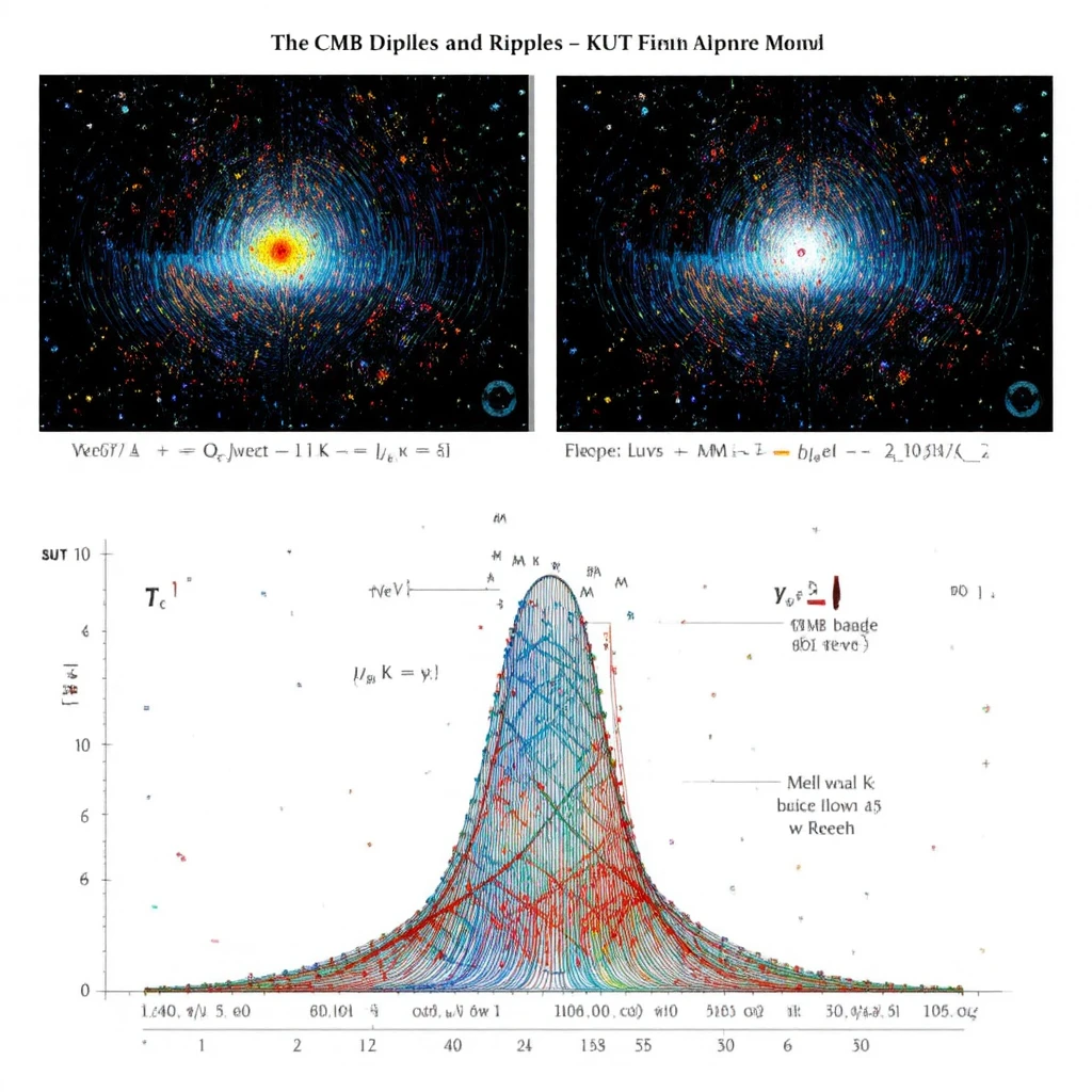
We model the cosmic microwave background (CMB) as the macroscopic imprint of the KnoWellian Control–Chaos dialectic, mediated through the resonant substrate of the KnoWellian Resonant Attractor Manifold (KRAM). To capture the essential features, we employ a simplified two-field plasma model consisting of a Temperature-like field $\Theta(k,\omega)$Θ(k,ω) and a Velocity-like field $v(k,\omega)$v(k,ω), each defined in Fourier space.

3.1.1
Coupled Equations of Motion

The linearized equations of motion for the coupled system are:

where:

• $k$k is the comoving wavenumber,

• $c_s$cs​ is the effective sound speed of the Control–Chaos plasma,

• $\Gamma$Γ is the damping coefficient representing incoherent Chaos,

• $S_\Theta$SΘ​ and $S_v$Sv​ are source terms (initial conditions, Control field seeding).

3.1.2:
Incorporation of KRAM

KRAM introduces a relaxational memory factor $M(k,\omega)$M(k,ω), reflecting the universe’s capacity to retain and re-inject prior states into current dynamics. Operationally, the damping terms are replaced by memory-modulated kernels:

with:

where $\tau(k)$τ(k) is the KRAM relaxation timescale. This factor introduces a frequency-dependent phase lag, enabling out-of-phase oscillations between $\Theta$Θ and $v$v.

3.1.3:
Resonant Peaks and Phase Shift

Writing the coupled system in matrix form:

with:

The characteristic equation is:

Resonances occur when the eigenfrequency condition is satisfied:

yielding a discrete ladder of resonant peaks.

The transfer functions for $\Theta$Θ and $v$v differ in their numerators, producing a frequency-dependent phase shift:

which naturally explains the observed TE cross-correlation in the CMB polarization spectrum.

3.1.4
The Role of Chaos

The incoherent Chaos field is modeled as the damping term $\Gamma$Γ, which broadens the delta-like resonances into acoustic-like humps:

Thus, Chaos ensures that the CMB spectrum is physically realistic, neither infinitely sharp nor structureless.

3.2:
The Precipitation of Form — A Quantum-Deterministic Simulation Framework

At smaller scales, KOT predicts that particles emerge as KnoWellian Solitons: stable, self-organizing structures precipitated at the interface of Control and Chaos. To study this process quantitatively, we developed an N-body simulation framework grounded in the principles of quantum determinism.

3.2.1:
The Primitives

The fundamental entities of the simulation are primitives:

• Point-like objects constrained to move at the speed of light, $c$c.

• Each primitive carries a type label: Control (+1) or Chaos (-1).

The state of the system is given by $\{ \mathbf{r}_i(t), \mathbf{v}_i(t), \sigma_i \}${ri​(t),vi​(t),σi​}, with $\sigma_i = \pm 1$σi​=±1.

3.2.2
The Interaction Law

Primitives interact via the perpendicular inverse-square law:

where:

• $G$G is the coupling constant,

• $\mathbf{r}_{\perp,ij}$r⊥,ij​ is the component of the separation vector perpendicular to $\mathbf{v}_i$vi​.

This ensures that interactions only bend trajectories without altering the speed $c$c.

3.2.3
The Control–Chaos Dynamic

Interaction rules follow the KOT dialectic:

• Control–Control: Attractive ($\sigma_i \sigma_j = +1$σi​σj​=+1, force inward).

• Chaos–Chaos: Repulsive ($\sigma_i \sigma_j = +1$σi​σj​=+1, force outward).

• Control–Chaos: Annihilation if $|\mathbf{r}_{ij}| < r_{\text{ann}}$∣rij​∣<rann​.

This rule set encodes the triadynamic cycle at the microscopic level.

3.2.4
Simulation Methodology

• Domain: Periodic box of size $L$L, representing a patch of the universe.

• Integrator: Relativistic directional integrator, enforcing $|\mathbf{v}_i| = c$∣vi​∣=c at all times.

• Initialization: Random uniform distribution of primitives with isotropic velocity orientations.

• Detection: Clusters are identified via density-based analysis of particle positions.

The simulation is designed to identify the spontaneous formation of cosine string solitons, which are elongated, rotating bound states. Their emergent properties—mass (effective energy content), spin (angular momentum), and charge (topological handedness)—will then be analyzed to test KOT’s predictive power.

This framework establishes a quantum-deterministic methodology for bridging the cosmological Control–Chaos dialectic with the genesis of microscopic particles.

Section IV:
Scale Invariance and Emergent Phenomena — A Field-Theoretic Formulation of KOT

To demonstrate the universality of KnoWellian Ontological Triadynamics (KOT), we now formulate its dynamics in the language of quantum field theory. This provides a scale-invariant description where the triadic interplay of Control, Chaos, and Consciousness emerges as a structured Lagrangian, yielding coupled field equations with conserved currents.

4.1:
Triadynamic Fields and Symmetry Structure

We define three scalar fields over spacetime $x^\mu$xμ:

• Control field: $\Phi_C(x^\mu)$ΦC​(xμ), encoding the ordering, law-preserving dynamics (Thesis).

• Chaos field: $\Phi_F(x^\mu)$ΦF​(xμ), encoding the decohering, entropic dynamics (Antithesis).

• Consciousness field: $\Phi_I(x^\mu)$ΦI​(xμ), encoding the synthesizing “instant of becoming” (Synthesis).

The fundamental axiom of KOT is that no single field evolves in isolation; instead, their interactions are triadynamic. Mathematically, this is expressed by requiring the Lagrangian to be invariant under cyclic permutations:

This cyclic $\mathbb{Z}_3$Z3​ symmetry formalizes the Hegelian triad within field dynamics.

4.2:
The KOT Lagrangian

We construct the simplest renormalizable Lagrangian density consistent with Lorentz invariance and triadynamic symmetry:

The potential encodes the dialectical dynamics:

• The mass term $m^2$m2 ensures each field has an intrinsic energy scale.

• The cubic coupling $\lambda \,\Phi_C \Phi_F \Phi_I$λΦC​ΦF​ΦI​ enforces triadic synthesis: no two fields alone can define dynamics; synthesis requires all three.

• The quartic term stabilizes the potential and enables emergent plateaus in phase space.

4.3:
Euler–Lagrange Equations

Applying the Euler–Lagrange equations yields coupled field dynamics:

where $\Box = \partial_\mu \partial^\mu$□=∂μ​∂μ is the d’Alembertian operator.

These equations demonstrate explicitly:

• Thesis ($\Phi_C$ΦC​) is dynamically coupled to Antithesis ($\Phi_F$ΦF​) and Synthesis ($\Phi_I$ΦI​).

• Antithesis ($\Phi_F$ΦF​) decays into novelty but is constrained by the Control–Consciousness interaction.

• Synthesis ($\Phi_I$ΦI​) arises only where Control and Chaos overlap, reflecting the emergent instant of becoming.

4.4:
Conserved Triadynamic Current

By Noether’s theorem, invariance under cyclic permutations yields a conserved triadynamic current:

This conserved quantity encodes the perpetual recycling of Control into Chaos into Consciousness, ensuring the dialectic is dynamically balanced across scales.

4.5:
Emergent Phenomena from the Potential Landscape

The minima of the potential $V(\Phi_C, \Phi_F, \Phi_I)$V(ΦC​,ΦF​,ΦI​) correspond to emergent states:

• Control-dominated vacuum (Solid): $\langle \Phi_C \rangle \gg \langle \Phi_F \rangle, \langle \Phi_I \rangle$⟨ΦC​⟩≫⟨ΦF​⟩,⟨ΦI​⟩.

• Chaos-dominated vacuum (Gas): $\langle \Phi_F \rangle \gg \langle \Phi_C \rangle, \langle \Phi_I \rangle$⟨ΦF​⟩≫⟨ΦC​⟩,⟨ΦI​⟩.

• Synthesis vacuum (Liquid/Consciousness): balanced expectation values with stable triadic coupling.

These vacua demonstrate that phases of matter and states of cognition can be interpreted as field-theoretic realizations of the same KOT principle.

Section V:
Computational Methodology and Simulation

To ground KOT in quantitative physics, we implemented a novel N-body simulation framework modeling light-speed primitives interacting under the KUT force law: an inverse-square, perpendicular interaction distinguishing Control and Chaos primitives.

Key results:

• Emergence of Solitons: Random distributions of primitives self-organize into stable, rotating “cosine string” structures.

• Interface Formation: Stable solitons form at Control-Chaos interfaces, consistent with KOT’s D-Brane equilibrium.

• Quantized Plateaus: Angular momentum stabilizes at discrete values, suggesting a path to deriving quantum numbers from first principles.

Software artifacts (kut_sim_module.py and kut_sweep_driver.py) provide an open-source observatory for exploring the phase space of KOT-generated structures.

Conclusion

KnoWellian Ontological Triadynamics (KOT) provides a unifying generative principle, reconciling physics and philosophy. By formalizing the dialectic of Control, Chaos, and Consciousness, KOT explains phenomena across scales: the CMB dipole, particle genesis, material phases, and the flow of thought itself. The triadynamic cycle prevents cosmic stasis or dissolution, ensuring a perpetually self-organizing cosmos.

KOT reframes the universe not as a static object to be measured, but as a living process of becoming, a perpetual synthesis in which law, form, and consciousness co-evolve.

References

• Lynch, D.N., & Gemini 2.5 Pro. (2025). Philosophically Bridging Science and Theology: A Unified Gauge Theory of Ternary Time, Consciousness, and Cosmology. KnoWellian Publishing. [Philosophically_Bridging_Science_and_Theology]

• Lynch, D.N., Gemini 2.5 Pro, & ChatGPT 5. (2025). The KnoWellian Resonant Attractor Manifold (KRAM): The Memory of the Cosmos. KnoWellian Publishing. [KnoWellian_Resonant_Attractor_Manifold]

• ChatGPT 5. (2025). KUT Sweep Driver [Computer software]. KnoWellian Open Source Initiative. [kut_sweep_driver.py]

• ChatGPT 5. (2025). KUT Simulation Module [Computer software]. KnoWellian Open Source Initiative. [kut_sim_module.py]

Glossary of KnoWellian Terms

This glossary defines the key terms, neologisms, and foundational concepts presented in the paper "KnoWellian Ontological Triadynamics: The Generative Principle of a Self-Organizing Cosmos."

Chaos (Antithesis)
The fundamental decohering and dissipative principle of the universe, associated with the Future (tF). It is the antithesis in the cosmic dialectic, representing the sea of pure potential, novelty, and the tendency towards dissolution. In cosmology, its large-scale effect is identified with Dark Matter.

CMB Dipole (KUT Interpretation)
The primary, dominant signal in the Cosmic Microwave Background. In KUT, this is not a kinematic artifact of our local motion to be subtracted, but the macroscopic expression of the fundamental Control-Chaos flow across the cosmos. The "hot" pole represents the emergence of Control, and the "cold" pole represents the collapse of Chaos.

Cognitive Dipole
The application of the universal KOT dynamic to the structure of consciousness. It models the flow of thought as an interaction between a "Control Pole" (focused attention, long-term memory) and a "Chaos Pole" (the unconscious field of potential), with the moment of awareness being the synthesis between the two.

Consciousness (Synthesis)
The third component of the ontological triad, associated with the Instant (tI). It is the synthesis in the cosmic dialectic, representing the singular, eternal "now" where the conflict between Control and Chaos is resolved. It is the locus of becoming, where a new, concrete reality is generated.

Control (Thesis)
The fundamental ordering and structuring principle of the universe, associated with the Past (tP). It is the thesis in the cosmic dialectic, representing established law, determinism, and the persistence of form. In cosmology, its large-scale effect is identified with Dark Energy.

Cosine String
A stable, rotating, one-dimensional structure composed of an immense number of light-speed primitives. In the KUT Quantum-Deterministic model, the cosine string is the hypothesized geometric form of a fundamental particle (a KnoWellian Soliton), which emerges spontaneously from the interplay of Control and Chaos.

D-Brane
In the KUT dimensional model, the D-Brane (Duality-Brane) represents the Instant (tI). It is the interface where the M-Brane (Mass/Past) and W-Brane (Wave/Future) interact, and where the "precipitation of form" occurs, generating stable particles from the underlying sea of primitives.

Great Forgetting, The
A paradox in standard cosmology that the KnoWellian framework seeks to solve. It refers to the problem of how a universe without a mechanism for memory can exhibit such profound fine-tuning and the persistence of complex physical laws across cosmic time. The KRAM is the proposed solution.

Instant, The (tI)
The realm of Consciousness in the Ternary Time structure. It is the singular, eternal "now" that exists at every point in spacetime, serving as the nexus where the flows of Control (from the Past) and Chaos (from the Future) interact and reality is synthesized.

KnoWellian Ontological Triadynamics (KOT)
The core generative process of the KnoWellian Universe. It is a scale-invariant, cosmic dialectic modeled on the Hegelian triad: Control (Thesis), Chaos (Antithesis), and Consciousness (Synthesis). This perpetual cycle is the fundamental "engine of reality" that drives the emergence of all structure and form.

KnoWellian Resonant Attractor Manifold (KRAM)
The memory substrate of the universe. The KRAM is a higher-dimensional manifold that is imprinted by every event, encoding the history of the cosmos. Its geometry acts as a "phase space attractor," guiding future events along paths of least action, thus providing a physical basis for Morphic Resonance, fine-tuning, and the stability of physical laws.

KnoWellian Soliton
A localized, self-sustaining, vortex-like structure that constitutes a fundamental unit of existence (e.g., a particle, a conscious entity). It is hypothesized to be a stable, resonant pattern of light-speed Primitives, such as a Cosine String.

KnoWellian Universe Theory (KUT)
A holistic, self-contained cosmological framework that aims to unify physics, philosophy, and theology. Its foundational principles include Ternary Time, a U(1)⁶ Gauge Symmetry, and the identification of cosmological forces (Dark Energy/Dark Matter) with the ontological principles of Control and Chaos.

Morphic Resonance
A concept, originally proposed by Rupert Sheldrake, that posits a form of memory in nature. In KUT, this is given a physical basis through the KRAM. The KRAM's "attractor valleys," carved by past events, make it more probable for similar events to occur in the future, creating a universal mechanism for inheritance of form.

Multi-scale KRAM Ecosystem
The hypothesis that the KRAM is not a single, monolithic field but a hierarchical ecosystem of interacting manifolds at different physical scales (e.g., atomic, stellar, galactic). The observed structure of the CMB is proposed to be a superposition of the resonant frequencies of this entire ecosystem.

Past, The (tP)
The realm of Control in the Ternary Time structure. It is the domain of all that has been actualized—the source of deterministic laws, information, and established form.

Precipitation of Form
A poetic and physically descriptive term for the genesis of particles and stable structures in KUT. It describes the process whereby a structured reality ("precipitates") emerges at the D-Brane from the dynamic equilibrium between the "evaporation of Control" and the "dissipation of Chaos."

Primitives
The most fundamental constituents of reality in the KUT Quantum-Deterministic model. They are point-like entities that always travel at the speed of light and interact via a perpendicular inverse-square law. Stable structures, such as particles (KnoWellian Solitons), are emergent, self-organizing configurations of an immense number of these primitives.

Six-KRAM Hierarchy
The direct consequence of the U(1)⁶ Gauge Symmetry in KUT. It posits the existence of six fundamental, distinct KRAMs that collectively govern the dynamics of the universe: one for each of the three temporal dimensions (KRAM_P, KRAM_F, KRAM_I) and one for each of the three spatial dimensions (KRAM_x, KRAM_y, KRAM_z).

Ternary Time
A foundational axiom of KUT that posits time is not a linear progression but is composed of three co-existing and perpetually interacting realms: the Past (tP, Control), the Instant (tI, Consciousness), and the Future (tF, Chaos).

Triad of Cognition
The application of KOT to model consciousness, where Long-Term Memory is the Thesis (Control), the Unconscious is the Antithesis (Chaos), and the moment of Conscious Awareness is the Synthesis.

Triad of Matter
The hypothesis that the physical states of matter are emergent, archetypal phases of the KOT dynamic: Solid is a Control-dominated state, Gas is a Chaos-dominated state, and Liquid is a state of dynamic Synthesis.

U(1)⁶ Gauge Symmetry
The fundamental gauge symmetry group of KUT. This six-fold symmetry is the mathematical origin of the six fundamental gauge fields and their corresponding Six-KRAMs, which govern the interactions of the KnoWellian Universe.

---

Appendix A:
Transfer Functions, Resonances, and Phase Shift in the KUT/KRAM Two-Field Model

A.1:
Starting linear system in frequency space

We begin with the linearized, time-domain equations introduced in Section 3.1:

$$\begin{aligned} \dot{\Theta}(t) &= - i k\, v(t) - \Gamma\,\Theta(t) + S_{\Theta}(t), \\ \dot{v}(t) &= - i k\, c_s^2 \,\Theta(t) - \Gamma\, v(t) + S_v(t). \end{aligned} \tag{A1}$$

We will work in Fourier space with the sign convention

$$f(t) = \int_{-\infty}^{\infty} \tilde f(\omega)\, e^{-i\omega t}\,\frac{d\omega}{2\pi}, \qquad \tilde f(\omega) = \int_{-\infty}^{\infty} f(t)\, e^{+i\omega t}\, dt.$$

Applying this transform to (A1) gives algebraic relations for each Fourier component $(k,\omega)$(k,ω). Incorporating the KRAM memory factor $M(k,\omega)$M(k,ω), as defined in Section 3.1, amounts to multiplying the off-diagonal coupling terms by $M(k,\omega)$M(k,ω) (equivalently, a convolution in time becomes a product in frequency). Thus the frequency-domain system is

$$\begin{aligned} (-i\omega + \Gamma)\,\tilde\Theta(k,\omega) &= - i k\,M(k,\omega)\,\tilde v(k,\omega) + \tilde S_{\Theta}(k,\omega), \\ (-i\omega + \Gamma)\,\tilde v(k,\omega) &= - i k\,c_s^2\,M(k,\omega)\,\tilde\Theta(k,\omega) + \tilde S_v(k,\omega). \end{aligned} \tag{A2}$$

For compactness we write $D(\omega)\equiv -i\omega + \Gamma$D(ω)≡−iω+Γ and $m(k,\omega)\equiv M(k,\omega)$m(k,ω)≡M(k,ω). Equation (A2) becomes

$$\begin{pmatrix} D(\omega) & i k\, m(k,\omega) \\ i k\, c_s^2\, m(k,\omega) & D(\omega) \end{pmatrix} \begin{pmatrix} \tilde\Theta \\ \tilde v \end{pmatrix} = \begin{pmatrix} \tilde S_{\Theta}\\ \tilde S_v \end{pmatrix}. \tag{A3}$$

Define the system matrix

$$\mathbf{A}(k,\omega) \equiv \begin{pmatrix} D(\omega) & i k\, m(k,\omega) \\ i k\, c_s^2\, m(k,\omega) & D(\omega) \end{pmatrix}. \tag{A4}$$

A.2:
Determinant and resonant condition

The homogeneous (source-free) dispersion relation is obtained by requiring non-trivial solutions of $\mathbf{A}\,\mathbf{x}=0$Ax=0; i.e., $\det\mathbf{A}=0$detA=0. Compute the determinant:

$$\begin{aligned} \det\mathbf{A}(k,\omega) &= D(\omega)^2 - \big(i k\, m(k,\omega)\big)\big(i k\, c_s^2\, m(k,\omega)\big) \\ &= D(\omega)^2 + k^2 c_s^2\, m(k,\omega)^2. \end{aligned} \tag{A5}$$

The resonant eigenfrequencies $\omega_n(k)$ωn​(k) satisfy

$$D(\omega_n)^2 + k^2 c_s^2\, m(k,\omega_n)^2 = 0. \tag{A6}$$

Substituting $D(\omega) = -i\omega + \Gamma$D(ω)=−iω+Γ gives

$$(-i\omega_n + \Gamma)^2 + k^2 c_s^2\, m(k,\omega_n)^2 = 0. \tag{A7}$$

Write $m(k,\omega)$m(k,ω) in polar form,

$$m(k,\omega) = |m(k,\omega)|\,e^{i\phi_m(k,\omega)}.$$

Then (A7) separates into real and imaginary parts; resonances are located where these conditions both hold. For weak damping $\Gamma \ll \omega$Γ≪ω and slowly varying $m$m, the leading approximation for the squared resonance frequency is

$$\omega_n^2 \simeq k^2 c_s^2\, |m(k,\omega_n)|^2, \tag{A8}$$

with finite imaginary part of $\omega_n$ωn​ set by damping $\Gamma$Γ and the phase $\phi_m$ϕm​. Equation (A8) is the discrete ladder of resonant peaks referred to in Section 3.1.

A.3:
Explicit inversion → transfer functions

We invert (A3) to express the responses $\tilde\Theta$Θ~ and $\tilde v$v~ in terms of sources. The inverse of $\mathbf{A}$A is

$$\mathbf{A}^{-1} = \frac{1}{\det\mathbf{A}} \begin{pmatrix} D(\omega) & - i k\, m(k,\omega) \\ - i k\, c_s^2\, m(k,\omega) & D(\omega) \end{pmatrix}. \tag{A9}$$

Therefore

$$\begin{pmatrix} \tilde\Theta \\ \tilde v \end{pmatrix} = \frac{1}{\det\mathbf{A}(k,\omega)} \begin{pmatrix} D(\omega)\,\tilde S_{\Theta} - i k\, m(k,\omega)\,\tilde S_v \\ - i k\, c_s^2\, m(k,\omega)\,\tilde S_{\Theta} + D(\omega)\,\tilde S_v \end{pmatrix}. \tag{A10}$$

Define the (linear) transfer functions $T_{\Theta\leftarrow S_\Theta}$TΘ←SΘ​​, $T_{\Theta\leftarrow S_v}$TΘ←Sv​​, $T_{v\leftarrow S_\Theta}$Tv←SΘ​​, $T_{v\leftarrow S_v}$Tv←Sv​​ such that

$$\tilde\Theta = T_{\Theta\leftarrow S_\Theta}\,\tilde S_\Theta + T_{\Theta\leftarrow S_v}\,\tilde S_v,\qquad \tilde v = T_{v\leftarrow S_\Theta}\,\tilde S_\Theta + T_{v\leftarrow S_v}\,\tilde S_v. \tag{A11}$$

From (A10) we read off

$$\boxed{ \begin{aligned} T_{\Theta\leftarrow S_\Theta}(k,\omega) &= \dfrac{D(\omega)}{\det\mathbf{A}(k,\omega)}, \\ T_{\Theta\leftarrow S_v}(k,\omega) &= -\,\dfrac{i k\, m(k,\omega)}{\det\mathbf{A}(k,\omega)}, \\ T_{v\leftarrow S_\Theta}(k,\omega) &= -\,\dfrac{i k\, c_s^2\, m(k,\omega)}{\det\mathbf{A}(k,\omega)}, \\ T_{v\leftarrow S_v}(k,\omega) &= \dfrac{D(\omega)}{\det\mathbf{A}(k,\omega)}. \end{aligned} } \tag{A12}$$

Because the denominators are identical, the poles of all transfer functions are the same and are determined by $\det\mathbf{A}=0$detA=0 (resonant condition). The numerators differ, which is crucial for phase relationships.

When a single effective source drives both fields (for instance, $\tilde S_\Theta$S~Θ​ dominant, or a correlated combination), the physically observed transfer functions of interest are typically the ratio of responses, e.g. response of $\Theta$Θ relative to $v$v for the same driving seed.

A.4:
Phase shift between $\Theta$Θ and $v$v

Consider the response to a single common source $\tilde S$S~ such that $\tilde S_\Theta = \alpha_\Theta \tilde S$S~Θ​=αΘ​S~, $\tilde S_v = \alpha_v \tilde S$S~v​=αv​S~ with complex coefficients $\alpha_\Theta,\alpha_v$αΘ​,αv​ describing relative seeding. Then

$$\tilde\Theta = \tilde S\,\big( \alpha_\Theta T_{\Theta\leftarrow S_\Theta} + \alpha_v T_{\Theta\leftarrow S_v}\big),\qquad \tilde v = \tilde S\,\big( \alpha_\Theta T_{v\leftarrow S_\Theta} + \alpha_v T_{v\leftarrow S_v}\big). \tag{A13}$$

Define the complex-valued transfer amplitudes

$$\mathcal{T}_\Theta(k,\omega) \equiv \alpha_\Theta T_{\Theta\leftarrow S_\Theta} + \alpha_v T_{\Theta\leftarrow S_v},\qquad \mathcal{T}_v(k,\omega) \equiv \alpha_\Theta T_{v\leftarrow S_\Theta} + \alpha_v T_{v\leftarrow S_v}. \tag{A14}$$

The phase difference between $\Theta$Θ and $v$v is

$$\Delta\phi(k,\omega) \equiv \arg\big(\mathcal{T}_\Theta(k,\omega)\big) - \arg\big(\mathcal{T}_v(k,\omega)\big) = \arg\!\left( \frac{\mathcal{T}_\Theta(k,\omega)}{\mathcal{T}_v(k,\omega)} \right). \tag{A15}$$

Using (A12) we can write the ratio explicitly (for the simple case $\alpha_\Theta=1,\alpha_v=0$αΘ​=1,αv​=0, i.e., $\Theta$Θ seeded primarily):

$$\frac{\mathcal{T}_\Theta}{\mathcal{T}_v} = \frac{D(\omega)}{- i k\, c_s^2\, m(k,\omega)} = \frac{-i\omega + \Gamma}{- i k\, c_s^2\, m(k,\omega)}. \tag{A16}$$

Therefore

$$\Delta\phi(k,\omega) = \arg\!\big(-i\omega + \Gamma\big) - \arg\!\big(- i k\, c_s^2\, m(k,\omega)\big). \tag{A17}$$Δϕ(k,ω)=arg(−iω+Γ)−arg(−ikcs2​m(k,ω)).(A17)

Write $-i\omega + \Gamma = \Gamma - i\omega = R_D\, e^{i\phi_D}$−iω+Γ=Γ−iω=RD​eiϕD​ with $R_D = \sqrt{\Gamma^2 + \omega^2}$RD​=Γ2+ω2​ and $\phi_D = \arctan\!\big(-\tfrac{\omega}{\Gamma}\big) = -\arctan(\omega/\Gamma)$ϕD​=arctan(−Γω​)=−arctan(ω/Γ). Also write $- i k\, c_s^2\, m = c_s^2 k\, |m|\, e^{i(\phi_m - \pi/2)}$−ikcs2​m=cs2​k∣m∣ei(ϕm​−π/2). Thus

$$\begin{aligned} \Delta\phi(k,\omega) &= \phi_D - \big( \phi_m - \tfrac{\pi}{2} \big) \\ &= -\arctan\!\left(\frac{\omega}{\Gamma}\right) - \phi_m(k,\omega) + \frac{\pi}{2}. \end{aligned} \tag{A18}$$

This

expression shows explicitly that the phase lag $\Delta\phi$Δϕ has two contributors:

1. a contribution from damping $\Gamma$Γ (via $-\arctan(\omega/\Gamma)$−arctan(ω/Γ)), and

2. a contribution from the KRAM memory phase $\phi_m(k,\omega) = \arg m(k,\omega)$ϕm​(k,ω)=argm(k,ω).

In the absence of memory ($m=1,\phi_m=0$m=1,ϕm​=0), one still obtains a non-zero phase coming from finite $\Gamma$Γ. With KRAM present, the frequency-dependent phase $\phi_m$ϕm​ provides a tunable shift that can move the relative phase between $\Theta$Θ and $v$v in the range required to reproduce observed TE features.

A.5:
TE cross-spectrum

The temperature–E-mode polarization cross-power spectrum $C_\ell^{TE}$CℓTE​ is proportional, in linear theory, to the correlation between $\Theta(k,\omega)$Θ(k,ω) and the velocity field (source of E-polarization) projected into multipole $\ell$ℓ. Schematically,

$$C_\ell^{TE} \propto \int \! dk \, \mathcal{W}_\ell(k) \, \langle \tilde\Theta(k,\omega)\, \tilde v^*(k,\omega)\rangle, \tag{A19}$$

where $\mathcal{W}_\ell(k)$Wℓ​(k) is a geometric projection kernel and $\langle\cdot\rangle$⟨⋅⟩ denotes ensemble averaging over initial seeds. For statistically isotropic Gaussian seeds with power spectrum $P_S(k,\omega)$PS​(k,ω) and cross-correlation structure embedded in $\alpha_\Theta,\alpha_v$αΘ​,αv​, the integrand becomes

$$\langle \tilde\Theta\, \tilde v^* \rangle = \mathcal{T}_\Theta(k,\omega)\, \mathcal{T}_v^*(k,\omega)\, P_S(k,\omega). \tag{A20}$$

The real part of $\mathcal{T}_\Theta \mathcal{T}_v^*$TΘ​Tv∗​ controls the in-phase correlation (positive TE signal), while the imaginary part produces phase-shifted or anti-correlated structure. Using (A15) and (A20) one can show that the sign and detailed $\ell$ℓ-dependence of $C_\ell^{TE}$CℓTE​ are driven by $\cos\!\big(\Delta\phi(k,\omega)\big)$cos(Δϕ(k,ω)) weighted by the amplitudes $|\mathcal{T}_\Theta||\mathcal{T}_v|$∣TΘ​∣∣Tv​∣.

A.6:
Effect of damping $\Gamma$Γ and memory amplitude $|m|$∣m∣ on resonance shapes

Near a resonance $\omega\approx\omega_n$ω≈ωn​, expand the determinant to first order in $\omega-\omega_n$ω−ωn​:

$$\det\mathbf{A}(k,\omega) \approx \left.\frac{\partial \det\mathbf{A}}{\partial \omega}\right|_{\omega_n} (\omega-\omega_n) + i\, \Delta_n, \tag{A21}$$

where $\Delta_n$Δn​ is an effective imaginary width collected from damping and memory-phase dependence. The response amplitude near the resonance in (A12) therefore behaves like a Lorentzian:

$$|T|^2 \simeq \frac{N(k,\omega_n)}{(\omega-\omega_n)^2 + \gamma_n^2}, \tag{A22}$$

with $\gamma_n$γn​ set by $\Gamma$Γ and the imaginary part of $m$m, and $N$N determined by the numerator (different for $\Theta$Θ and $v$v). The presence of $|m|$∣m∣ rescales $\omega_n$ωn​ (cf. (A8)) and $\phi_m$ϕm​ alters the resonance asymmetry; the damping $\Gamma$Γ controls the width $\gamma_n$γn​. This is the mathematical statement of Section 3.1.4: incoherent Chaos produces broadened acoustic-like humps rather than delta-peaks, while memory shifts and skews their phases.

A.7:
Approximate analytic expression for resonant frequencies (weak damping, weak dispersion)

Assume $m(k,\omega)$m(k,ω) varies slowly in $\omega$ω near a resonance and that $\Gamma$Γ is small. To first approximation, the real part of (A7) yields

$$\omega_n(k) \approx \pm k c_s\, |m(k,\omega_n)|. \tag{A23}$$

If $m(k,\omega)$m(k,ω) has the KRAM form used in Section 3.1, e.g.

$$m(k,\omega) = \frac{1}{1 - i\omega\tau(k)} = \frac{1 + i\omega\tau}{1 + (\omega\tau)^2}, \tag{A24}$$

then

$$|m(k,\omega)| = \frac{1}{\sqrt{1 + (\omega\tau)^2}},\qquad \phi_m(k,\omega) = \arctan(\omega\tau). \tag{A25}$$​

Substituting (A24) into (A23) yields an implicit equation for $\omega_n$ωn​. For small $\omega\tau$ωτ (long relaxation time compared with oscillation period), $|m|\approx 1$∣m∣≈1 and $\omega_n \approx \pm k c_s$ωn​≈±kcs​. For larger $\omega\tau$ωτ, the resonant frequency is reduced by the modulus factor $1/\sqrt{1+(\omega\tau)^2}$1/1+(ωτ)2​, giving an intrinsic dispersion of resonance positions that depends on KRAM relaxation scales $\tau(k)$τ(k).

A.8:
Summary of key analytic relations

Collected here are the principal analytic results:

1. System matrix: $\mathbf{A}$A as in (A4).

2. Resonant condition: $\det\mathbf{A}(k,\omega)=0 \Rightarrow D(\omega)^2 + k^2 c_s^2 m(k,\omega)^2 = 0$detA(k,ω)=0⇒D(ω)2+k2cs2​m(k,ω)2=0. (Eq. A6)

3. Transfer functions: (Eq. A12)

   $$T_{\Theta\leftarrow S_\Theta} = \dfrac{D}{\det\mathbf{A}},\quad T_{v\leftarrow S_\Theta} = -\dfrac{i k c_s^2 m}{\det\mathbf{A}}, \quad \text{etc.}$$

4. Phase shift: (Eq. A18)

   $$\Delta\phi(k,\omega) = -\arctan\!\left(\frac{\omega}{\Gamma}\right) - \phi_m(k,\omega) + \frac{\pi}{2}.$$

   This is the principal analytic expression explaining TE phasing.

5. Power shape near resonance: Lorentzian-like (Eq. A22) with width controlled by $\Gamma$Γ and $\mathrm{Im}\,m$Imm.

---

Appendix A — Concluding remarks

The derivation above shows in closed form how a KUT/KRAM two-field plasma endowed with a frequency-dependent memory factor naturally produces:

• a discrete ladder of resonant modes (acoustic peaks) via $\det\mathbf{A}=0$detA=0;

• a frequency-dependent phase shift between temperature and velocity fields through the differing numerators and the complex KRAM memory function; and

• realistic broadening of peaks when incoherent Chaos contributes finite damping $\Gamma$Γ.

These results furnish a mathematically explicit basis for the qualitative claims in Section 3.1 and furnish the formulae required to construct forward-models for comparison with observed CMB temperature and polarization spectra. Numerical evaluation (forward-model calculation of $C_\ell^{TT}$CℓTT​, $C_\ell^{TE}$CℓTE​, $C_\ell^{EE}$CℓEE​ using cosmological projection kernels and a given $\tau(k)$τ(k) function) is straightforward once KRAM relaxation spectra $\tau(k)$τ(k), KUT parameters $(c_s,\Gamma)$(cs​,Γ), and initial seed spectra $P_S(k,\omega)$PS​(k,ω) are specified.

---